Never would have imagined that the laws of physics would be so important in a world where virtualization is the new normal.
Data Locality is Important
Data Locality, refers to the ability to move the computation close to the data. This is important because when performance is key, IO quickly becomes our number one bottleneck. Data access times vary from milliseconds to seconds because of many factors like hardware specifications and network capabilities.
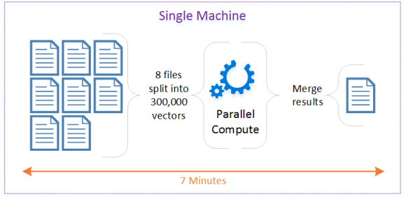
Let’s explore Data Locality through the following Scenario. I have eight files containing data about multiple trucks, and I need to Identify trips. A trip consists of many segments, including short stops. So if the driver stops for coffee and starts again, this is still considered the same trip. The strategy depicted below is to read each file and to group data points by truck. This can be referred to as mapping the data. Then we can compute the trips for each group in parallel over multiple threads. This can be referred to as reducing the data. And finally, we merge the results in a single CSV file so that we can easily import it to other systems like SQL Server and Power BI.
The single machine configuration results were promising. So I decided to break it apart and distribute the process across many task Virtual Machines (TVM). Azure Batch is the perfect service to schedule jobs. Building on my initial approach, I started by using Append Blobs to construct my vectors. This approach didn’t turn out the way I expected so I pivoted and used Azure Table Storage instead. This allowed me to partition my data effectively. At the time, this seemed like the best idea, because tables are optimized for many parallel operations on many partitions at once.
For a short amount of time, the architecture shown below was promising. However, I rapidly understood that physics didn’t agree with me.

End-to-End Workflow
- Each Task pulls a source CSV files from Azure Blob Storage
- The Task groups data points by truck, batches them by 100 and persists them to Azure Table Storage
- The task produces a list of all Azure Table Partition Keys generated for each source CSV file
- Each Task pulls an index from Azure Blob Storage
- Each Task reads partitions from Azure Table Storage and identifies trips
- Once trips are identified, a Task merges the results and pushes it back to the origin Azure Blob Storage
Why isn’t This the Best Approach?
Physics. I mentioned this a few of times now, so let’s delve into why physics matter in this scenario.
Every time we make a request over the network, we are challenged by the speed of light, and by the physical limitations of each hardware component that is part of the overall infrastructure. These are constants that we need to consider when we build our software solution.
Let’s do the math
As you read through the delays, keep in mind that they are distributed across 8 Task Virtual Machines (TVM).
- Downloading a 50 MB file was fast, so let’s be generous and say 10 seconds.
- Then each file produced about 150,000 vectors. With a total of 300,000 unique vectors across all files.
- Persisting the data to Azure Table Storage put pressure on the service and resulted in long HTTP requests. These ranged from 10ms to more than 400ms.
- Reading vectors back out of Azure Table Storage by PartitionKey also ranged from 10ms to 500ms
- Compute was negligible
- Uploading back to Azure Blob Storage was very quick, say less than a minute.
In the end, my process went from completing in 7 minutes to taking just a bit more than 50 minutes. And the reason for this is that I was moving large amounts of data from storage to the compute.
What Should I have Considered
The best approach is to bring the compute to the data. This drastically reduces the network tax and allows us to benefit from Data Locality. Right, this sounds great in theory, but how do I execute code against storage in Azure?
Your first option is to explore a Big Data solution like Hadoop. This ecosystem is built around Data Locality. When working with Petabytes of data, it doesn’t make sense to move it around all the time, so we bring the compute to the data and extract the results. This is ideal for many scenarios like batch processing and predictive analytics.
The second option that comes to mind is for real-time scenarios where Service Fabric really shines. It brings data and business logic together. This is especially important in scenarios where time is a significant factor. If the trucks could stream data to Azure using IoT Suite, Event Hubs or direct HTTP calls to in memory objects (Actors) hosted on Service Fabric, trips would be identified instantly and could, then be pushed out to other systems for batch processing, machine learning, business intelligence and dash boarding.